The temporal database is a database that can keep information on time when the facts represented in the database were, are, or will be valid. We briefly described major concepts of temporal databases and discussed types of queries that such databases can support in part 1 of this article series. The content of part 1 is essential for understanding the part 2.

In this part 2 we discuss what kind of aggregates can be obtained from a temporal database and how to express these aggregations in the SQL language. The examples in the part 2 are based on table definitions and data from part 1 of this article.

Before we start with discussion of aggregates, we remind that a row of the temporal table has a period of validity represented as a pair of timestamps. The lower boundary (start of the period is included into period and the upper boundary (the end of the period) is not. A validity period is associated with every value, but we assume that periods of all attributes of a row are the same. We also assume that the periods represent valid time (rather than system time), that is, the time when the information was or is correct in the reality but not necessarily stored in the database.

Note: If you want to restart with a clean database, the code that creates the structure and data from Chapter 1 is located in this file on the Simple Talk site.

Why Aggregates are Special?

An aggregate is a value calculated using column values from several rows. Usually aggregates represent information about large amount of data in a compact form, typically as a single value that is easy for human interpretation.

A single numeric value of an aggregate may represent thousands or even millions of values in the OLAP queries. The most common aggregates defined in the SQL standard are count, sum, avg (average), max, and min.

As discussed in the part 1, any non-temporal query, of course, including queries containing aggregates, can be easily converted into a temporal point-in-time query. So, what is the problem with aggregates?

As we mentioned in part 1, a point-in-time query produces non-temporal output because rows of the result have associated periods. Therefore, the output of such query is not a temporal table. To obtain the full power of SQL, we need to combine query output with other temporal tables in more complex queries. Also, sometimes aggregated values are naturally associated with certain periods in the real world.

However, an attempt to calculate aggregates for a period may result in unexpected and/or misleading results. For example, the following query sums the salary of each person as many times as there are rows for that person that overlap with the desired target period:

The output of this is silly, first, because inflates the salaries of people who changed salary amounts as time goes on. Second, there is little value to add such data together in the first place.

A more meaningful result can be obtained if we split the target period (the whole year) into smaller periods such that the value of salary does not change during any small period. The result will contain a separate row for each small period.

In general, the period associated with a value is calculated as intersections of all validity periods used to calculate the output value. This does not produce any difficulties for joins, unions and other relational operations that combine small number of arguments (usually two). However, for aggregates combining thousands or millions of rows the calculation of periods becomes challenging:

• It is computationally complex.
• The result, most likely, will contain huge number of tiny periods. So, it will not be compact anymore and hence will not be easy for humans.

We need to define temporal aggregates that produce a single value for a given period even if the values being aggregated have different validity periods not necessarily containing the target period. The target period may be specified as a part of a query or calculated from other rows (for example, joined from another table). In both cases the period for the aggregate is not based on periods of aggregated values.

For example, the company management may be interested in average salary of employees during the second quarter of 2023. However, the salary of Eja has been changed on April 20, so the function avg(salary) will produce wrong value, based on when the salary was changed.

Management does not want two values: one before April 20 and another after, just a single value is needed. Instead of averaging the values stored in the table, we compute a single value characterizing the salary during the period requested in the query (that is, second quarter) for each employee and then compute average of these values.

Aggregating Temporal Data

To make aggregation more useful we need to define more carefully how to calculate the aggregate values.

Although it is possible to express these calculations directly in SQL, we would like to define new aggregate functions that produce single number of any target period [query_ts, query_te] specified in a query and passed to the aggregate function as an argument.

Our aggregate functions should return the same result as the corresponding SQL function if the values of the column do not change during the query period. In particular, if the query period is a point, then our functions will return the same output as standard SQL functions.

Further, if the intersection of a row period with the query period is smaller than the query period, we use only a fraction of the aggregated value. For example, in some scenarios, if the duration of the query period is 3 months, but a person left the project after one month, we would like to count this person as 1/3, rather than 1 against the cost of a project. If this person worked on another project for remaining two months, we’ll count 2/3 to the second project.

Similarly, if a person has salary S₁ for two months and S₂ for remaining month of the target period, we use the value S₁*2/3+S₂*1/3 as a single number representing the salary of the person during the whole period. Of course, this value is not precise, but it gives a reasonable estimation.

So, we need to calculate fractions. Unfortunately, some of widely used calendar periods may have varying duration: neither months nor quarters are equal, and even leap years give us different lengths of year. This makes our function approximate, but we must measure duration of periods in the same units no matter how long or short periods are. Fortunately, it is possible to express duration of any period, even down to the second.

To do this, we will use SQL function extract with a first parameter of(epoch …) (that returns the duration of an interval in seconds) to calculate durations of periods. For example, the duration of the query period in seconds is calculated by the following expression:

Note that the difference of timestamps is an interval in the PostgreSQL type system. The duration in seconds may be very large for long periods, but we need only ratio of durations which will be always less than 1.

Similarly, we can calculate the duration of the intersection, using greatest, least, and EXTRACT functions, take some precautions to avoid a zero_divide exception, multiply by the value of an aggregated column and use all that as an argument for SQL sum function.

To avoid long constant values of timestamps and to make queries more readable, we define psql variables that contain the start and the end of the target query period:

These variables are proceeded with ‘:’when used in queries. Please note that the values are substituted before the query is sent to the server (so, they are NOT bind variables). For example, the string

is sent to the DBMS server as

Editor note: in DBeaver, I was able to use the following:

For more information on the settings required, this stackoverflow post covers it well.

If your client does not support any similar kind of variables, you can just substitute them with constants. We are now ready to write an SQL query that computes an aggregated value for the target period:

The output of this query is:

The query above computes only one aggregate, but we need much more in our examples. To make subsequent queries shorter, we wrap the code into PostgreSQL functions and define PostgreSQL user-defined aggregates temporal_sum, temporal_count, and temporal_avg. These functions have four additional arguments specifying the boundaries of the validity period of the aggregated value and the query period.

The complete code of these aggregates can be found in the appendix.

All queries below produce temporal results, that is, each row of the result has associated pair of timestamps. However, to avoid too long rows, we do not include these timestamps into the list of output columns if the periods for all output rows are the same.

Our first query uses temporal aggregates with GROUP BY name clause. Names are unique in our table, so such query would include exactly one row into each group and the value of count would be 1.

This returns:

The number of returned rows (6) is correct, but one of the values for count is 0.5. This is because Antti joined the company right in the middle of the period of the qery. So, our aggregate calculates a weighted average for each business key and then compute sum, average, or count.

A more interesting (from a business perspective) query calculates the aggregates with grouping by project:

This returns:

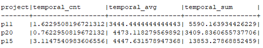
This output shows how intensive (and how expensive) the projects are. The non-integer values for count may look contra-intuitive. However, if a person worked for 3 different projects during 3 months, our calculation will show 1/3 for each project and the total 1 for all 3 projects. Counting this person as 1 for each project would be misleading. Our calculation is not cutting the body of a person into fractions, it only shows that the person’s effort wat not fully dedicated to a single project.

The reader is encouraged to run this query for different query periods. The results will be only slightly different. If you expect that salary for period of 4 months will be approximately 2 times lagrger than for 2 months, this will not happen. The reason is that the salary in the table is per month, no matter how long the query period is.

How to calculate the total to be paid during the period? We have yet another aggregate, temporal_accum for that. This aggregate has one more argument: the interval of time for which the aggregated value is specified. In our case this interval is equal to one month because the table stores salary per month. If you changed that to annual or per week salalry, the interval must be one year or one week.

Consider completely different application domain. Let the table store values of speed (for example, GPS readings) expressed in kilometers (or miles) per hour, then the interval will be one hour and the aggregate temporal_accom will calculate the distance covered during the query period.

Let’s now return to our table emp_temporal. The following query calculates the totals for the query period:

This returns the following.

The first column accumulates the value 1 with the interval on month, so the values in this column are mythical person-months spent on the project during the query period.

According to the title of a famous book ‘The Mythical Man-Month’ by F. Brooks, the man-months were mythical in 1970-ies. Man-months are now renamed with the more appropriate person-months, but we think they are still mythical. Note that the unit of measure is also important here: if we replace the interval parameter with one year instead of month, we’ll get mythical person-years.

Our last query calculates aggregates for each quarter of 2023. There is no query period for this query because different rows must have different periods (quarters). Therefore, the periods for which the aggregates are calculated are coming from the database (table qu), rather than from query parameters (as in previous queries).

Our example tables do not contain any data for periods outside of 2023. In more realistic scenarios we should also explicitly specify the query period so that only quarters of required year would be selected.

We rounded all values except count using ceil function to make the output more readable, which rounds up the specified number where needed. The value of temporal_count is rouned using the function round.

This should return something like this:

The above query produces an overall summary for all projects. Of course, GROUP BY q.code, e.project clause will produce more detailed data on each project per quarter. Probably ORDER BY clause is also welcome to make the management completely happy.

All values produced by our aggregates are approximate. The reason is that different months differ in duration. Of course, the problem is in the calendar rather than in the implementation of aggregates. So, these aggregates are probably good for planning, reporting, and analytics, but not for accounting.

We discussed count, sum, and avg functions so far. What about in and max? These two functions are much easier: the values from all rows that overlap with the target period produces meaningful result.

Conclusions

Aggregation in temporal databases over time periods requires special attention. Straightforward use of standard SQL aggregates may produce unexpected or incorrect output.

The aggregates described in this article produce compact output that have associated meaningful periods of validity. Consequently, these aggregates can be used in queries producing temporal tables.

Finally, although our implementation uses PostgreSQL-specific features, we tried to reduce dependency on the specific DBMS.

References

This section is identical to the corresponding section in the part 1 of this article.

During first decades of research on temporal database a complete bibliography was maintained. More information on this bibliography is available in [1]. The book [2] highlights the major outcome of that research. A systematic presentation of theoretical viewpoint on temporal databases can be found in [3].

An article [4] provides an overview of temporal features in SQL Stanard 2011 (that weren’t significantly changed in subsequent editions of the Standard). It also contains rationale for decisions made in the Standard.

One of several practical approaches to implementation of temporal features is described in [5]. The authors introduce asserted time dimension and describe advantages of bi-temporal data model based on effective time dimensions.

An article [6] introduces an alignment operation that provides an extension of relational algebra supporting temporal operations for one-dimensional time.

Finally, an emotionally rich annotated bibliography is available at [7].

1. Michael D. Soo. 1991. Bibliography on temporal databases. SIGMOD Rec. 20, 1 (March 1991), 14–23. https://doi.org/10.1145/122050.122054
2. Abdullah Tansel, James Clifford, Shashi Gadia, Sushil Jajodia, Arie Segev, and Richard T. Snodgrass (editors). Temporal Databases: Theory, Design, and Implementation. 1993.
3. C. J. Date, Hugh Darwen, Nikos Lorentzos. Time and Relational Theory, Second Edition: Temporal Databases in the Relational Model and SQL. 2nd edition, 2014.
4. Krishna Kulkarni and Jan-Eike Michels. “Temporal Features in SQL:2011”. SIGMOD Record, September 2012
5. Tom Johnston and Randall Weis. Managing Time in Relational Databases: How to Design, Update and Query Temporal Data. 2010.
6. Anton Dignös, Michael H. Böhlen, and Johann Gamper. 2012. Temporal alignment. In Proceedings of the 2012 ACM SIGMOD International Conference on Management of Data (SIGMOD ’12). Association for Computing Machinery, New York, NY, USA, 433–444. https://doi.org/10.1145/2213836.2213886
7. Temporal Databases Annotated Bibliography. https://illuminatedcomputing.com/posts/2017/12/temporal-databases-bibliography/

Appendix

This appendix contains the code of the temporal aggregates for PostgreSQL. A PostgreSQL aggregate consists of state variable and few functions. We use function sfunc that is invoked for every aggregated row and calculates new value of the state. For all functions except temporal_avg the final value of the state is just the value to be returned by the aggregate function. The state of temporal_avg consists of values for sum and count, so one more function is needed to return the final value of the aggregate function.

The code is also available here on the Simple Talk site.