Microsoft Fabric is a new centralized, AI-powered cloud data platform hosted by Microsoft. It combines several services of the existing Azure Data Platform – such as Azure Data Factory – with Power BI, while also introducing new services. It’s tempting to compare Microsoft Fabric with Azure Synapse Analytics since Synapse also bundles different services together, but Fabric is so much more. In contract with Synapse, Fabric is a software-as-a-service (SaaS) platform providing you with many low-code to no-code data services.

This doesn’t mean no code has to be written. On the contrary, in this article we’re going to focus on two services of Fabric: the lakehouse and the warehouse. The first one is part of the Data Engineering experience in Fabric, while the latter is part of the Data Warehousing experience. Both require code to be written to create any sort of artefact. In the warehouse we can use T-SQL to create tables, load data into them and do any kind of transformation. In the lakehouse, we use notebooks to work with data, typically in languages such as PySpark or Spark SQL.

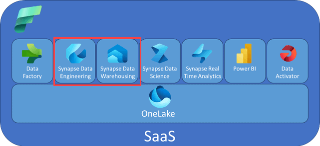
Figure 1: high-level overview of the services in Microsoft Fabric

ALT: a diagram displaying all available services in Fabric, with the Onelake storage layer beneath them

For an overview of all the available services/experiences in Fabric, check out the article Microsoft Fabric Personas.

If we can create tables and work with data in both the lakehouse or the warehouse, how do we choose between the two? When would you use one or the other? The answer is – as always – it depends. In this article, we’re going to present you with the advantages and disadvantages of each service and everything else you might take into consideration to make an informed decision about which service might be best suited for your use case.

Microsoft Fabric behind the Scenes

Before we start, let’s take a look first at how Microsoft Fabric works. For example, how is data stored in Microsoft Fabric? The answer is quite simple: everything is stored in the OneLake storage layer. This is a logical data lake build on top of Azure Data Lake Storage Gen2. It acts as a wrapper around this storage. Microsoft commonly refers to OneLake as “OneLake is the OneDrive for your data”. This means that in reality you might be using one or more Azure Data Lake storage accounts depending on your set-up and which regions you use, but you will perceive it as one single storage. As mentioned before, Fabric tries to centralize as much as it can. A benefit of this is that one service can read data stored by another service. For example, if you create a table in a lakehouse, you can query this table from a warehouse. This is known as the OneCopy feature.

Another interesting fact about storage is that all tables you create in the warehouse and in the lakehouse are delta tables. Delta is an open-source format that applies a transaction log on top of Parquet files. In other words, all table data is stored in Parquet files (these are well-compressed files where data is stored using a columnstore format). However, Parquet files are immutable, which means they cannot be updated after they are written to storage. Every time you insert, update or delete a record in a table, a new Parquet file has to be written out. The delta format manages a transaction log alongside all those Parquet files, guaranteeing ACID compliance just like in relational databases. In short, thanks to the delta format, we can use Parquet files to store our data but it all works similar to a regular relational database such as SQL Server.

When we look at how a table is stored in OneLake, we can see two folders:

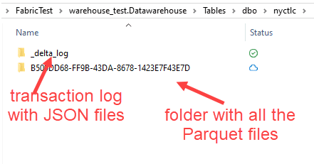
Figure 2: Delta table with transaction log and Parquet files

ALT: delta table in the storage layer. One folder for the transaction log, one folder for the Parquet files

In the _delta_log folder we can see the whole transaction log of the table:

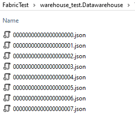
Figure 3: Transaction Log of the Delta Table

ALT: transaction log of a delta table, showing 8 different transactions

In the other folder, we can see a whole bunch of Parquet files. They contain the data of the table through various points in time (new files can be created after each transaction).

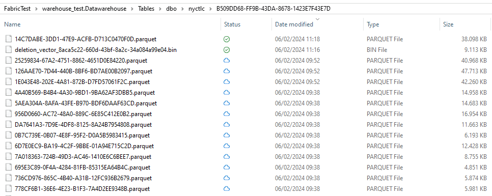
Figure 4: The different Parquet files of a Delta Table

ALT: a folder with a bunch of Parquet files. Displayed is also a deletion vector file.

The folder also contains a deletion vector, which is an optimization technique to handle deletes more efficiently.

Now we know how data is stored, but how is the compute managed in Fabric? The driving force behind everything in Fabric are the capacities. A capacity is a compute resource and is designated with a scale. The lowest capacity is an F2, the next one is F4, then F8 all the way up to F2048. Every time something wants to use compute, the capacity is used. It doesn’t matter if it is a warehouse, a data factory pipeline, or a real-time stream, it all uses the same capacity.

In the Microsoft Fabric portal (which is the same as the one used for Power BI), you can create workspaces and you can assign a capacity to that workspace.

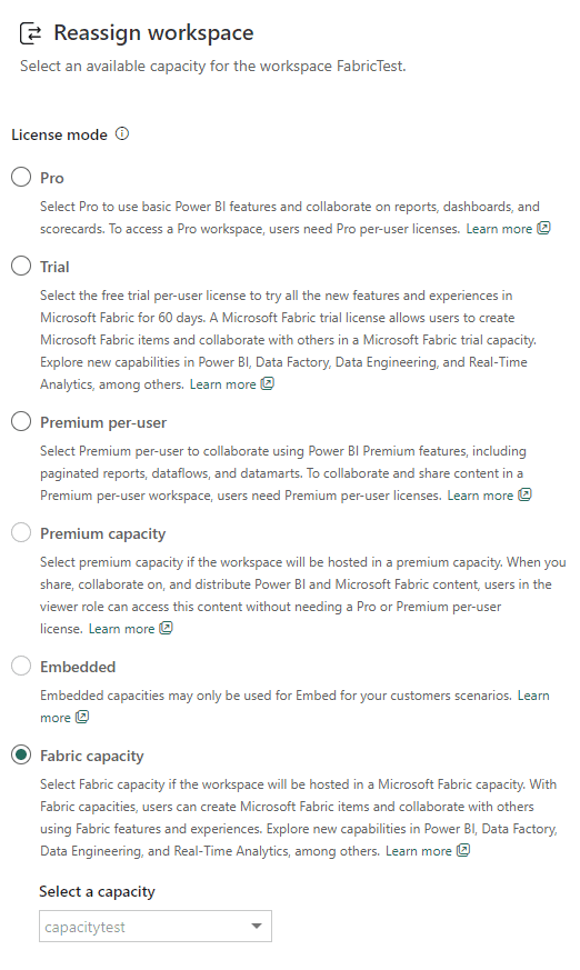
Figure 5: Assigning a Fabric capacity to a workspace

ALT: the list of options when assigning a capacity to a workspace

At the time of writing, there’s also a free trial of Fabric available. This trial capacity is equivalent with an F64. There are three methods of purchasing Microsoft Fabric:

• You provision an F-SKU through the Azure Portal. This capacity can be paused. You will be billed for the time the capacity is running. The capacity can be scaled up and down when needed. This is pay-as-you-go pricing. You can learn more about this option in the article What are Capacities in Microsoft Fabric?.
• You can also buy a reserved capacity. You pay for a reserved number of CU (capacity units) up front. Say for example that you buy an F4 with reserved pricing for the whole year. But the capacity that you’ve been running the whole time is an F8. This means that 4 capacity units will be subtracted from the total of 8, so you only pay for 4 capacity units with pay-as-you-go pricing. If you don’t scale up and only use F4 for the whole year, you’d pay nothing extra. So think of the reserved capacity units as some sort of “voucher” that you can use to get capacity units at a lower cost. More info can be found in the documentation.
• The last option is to buy Power BI Premium. With Power BI Premium, you get a fixed capacity that you can assign to workspaces, and you also get all of the Fabric capabilities with it. A P1 Premium capacity is equivalent with an F64, a P2 with an F128 and so on.

The following table gives an overview of the SKUs and indicative prices for the pay-as-you-go options:

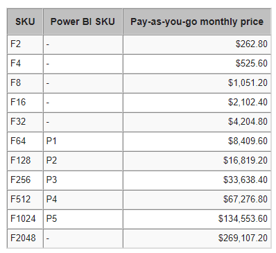
Figure 6: Price overview for Fabric

ALT: a table with the capacities from F2 till F2048 along with prices

A P1 Premium capacity is around $5,000, so it is considerably cheaper than an F64 if you would keep it running all the time. Only consider the pay-as-you-go option if you can pause the capacity for longer periods of time.

To conclude this section: every compute service in Microsoft uses the OneLake storage layer to store data (and in the case of the warehouse and the lakehouse it’s both delta tables), and they also use the same capacity for compute resources. So if both compute and storage are the same, what is the difference between the lakehouse and the warehouse?

The Warehouse versus the Lakehouse

The Warehouse

Even though the storage layer is completely different from SQL Server, a lot of effort has been made to make the warehouse have the look and feel of the old ‘n trustworthy relational database. When you create a warehouse in Fabric, you’ll be taken to the following screen:

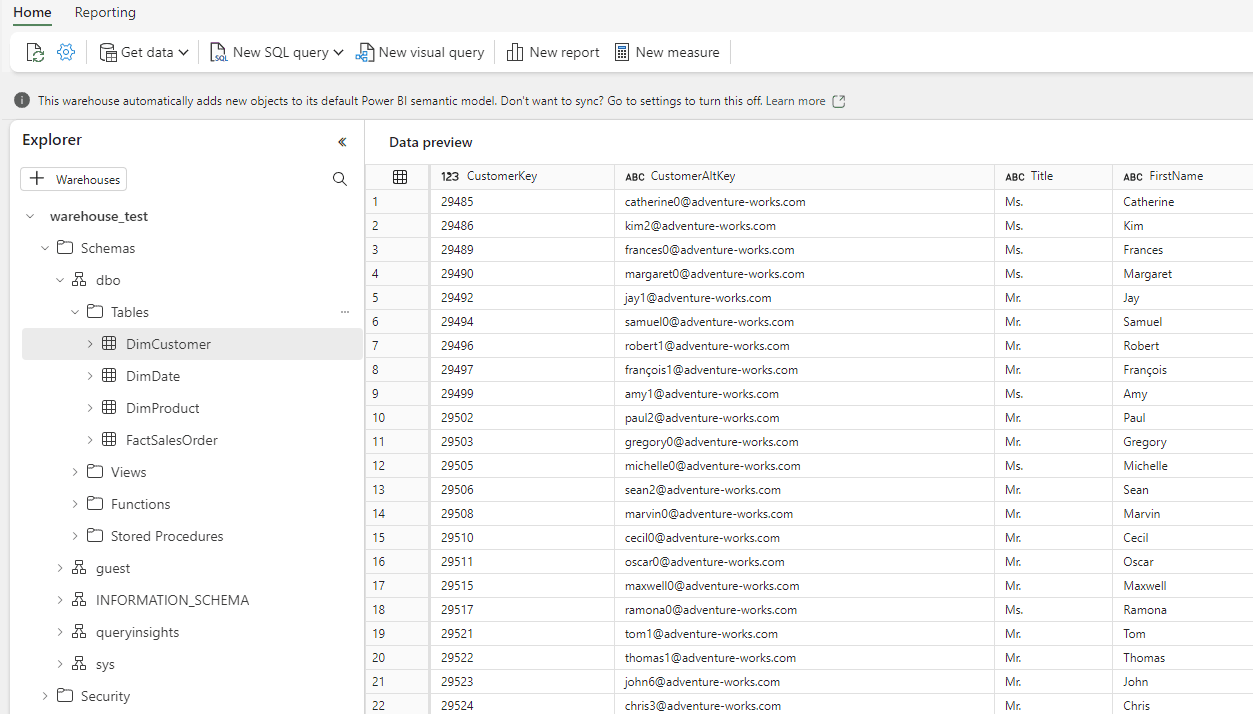
Figure 7: Warehouse Editor in Fabric

ALT: the Fabric warehouse editor in the browser. On the left there’s an explorer, on the right a data preview pane.

You can see familiar objects from SQL Server present: the dbo schema, tables, views, functions, and stored procedures. Working with the warehouse in Fabric is very similar to “traditional data warehousing” using a database like SQL Server or Azure SQL Database. Once data has been loaded into tables, you will write (mostly) the same T-SQL as we’ve been doing for the past years/decades.

However, not everything is supported (yet). For example, the TRUNCATE TABLE statement isn’t available, as well as identity columns, temporary tables, and the MERGE statement. Hopefully many limitations will be lifted in the future. You can find an overview of the current limitations in the documentation. Primary keys, foreign keys and unique keys are supported, but at the moment they’re not enforced. It can still be useful to create them, as it allows the query engine to create more optimal plans and because some BI tools use constraints to automatically create relationships. More info can be found here.

Ingesting Data

Before we start writing SQL, we must ingest data first. There are several options available:

• Data Pipelines. These are very similar to Azure Data Factory pipelines. They are a low-code to no-code experience for copying data to a destination (in this case the warehouse), or for orchestrating various other tasks. You can schedule pipelines for automatic data retrieval.

Figure 8: Sample Pipeline in Fabric

ALT: a sample pipeline in Fabric consisting of 4 activities

• Dataflows. These are very similar to Power BI dataflows. Both use the Power Query engine, but dataflows in Fabric can write to several possible destinations. Unlike data pipelines, you can actually see the data you’re working with, making them ideal for “citizen developers”. You can define a refresh schedule for a dataflow, or you can trigger them from a pipeline.

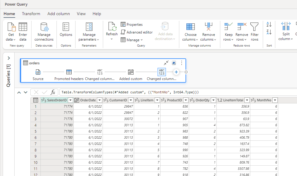
Figure 9: Fabric Dataflow with sample data

ALT: an example of a Fabric Dataflow, with data in preview

• COPY T-SQL statement. With the COPY INTO statement, data stored in Parquet files or in CSV files can be loaded into a warehouse table. Currently only Azure Data Lake Storage or Blob accounts are supported as an external location.
• Selecting data from other workspace sources. As mentioned before, thanks to the OneCopy principle, data can be read from other warehouses or lakehouses. You can use the 3-part naming convention database.schema.table to reference a table in another warehouse/lakehouse. Using SQL statements such as CREATE TABLE AS SELECT (CTAS), INSERT INTO or SELECT INTO, we can retrieve data from other sources (or from within the same warehouse), transform it and then write the results to a table.

People who have been working with the SQL Server platform or with the Azure Data Platform should be familiar with most of the options available to ingest data. In fact, existing code should be able to be migrated to the Fabric ecosystem, keeping in mind that there are still some limitations to the T-SQL supported in Fabric.

For more information about the data ingestion options, check out the documentation or the article Microsoft Fabric Data Ingestion Methods and Tools.

Transactions

Thanks to the transaction log of the delta tables, but also thanks to an internally managed transaction log, the warehouse is fully ACID-compliant. Only the snapshot isolation level is supported. Transactions that span across different databases in the same workspace are supported.

More information about transaction in the warehouse can be found here.

Security

The same access controls that exist in SQL Server are available in the Fabric warehouse as well. You can use GRANT and DENY for granular object or column level security for example. For more fine-grained access, you can use row-level security or data masking. The documentation page Security for data warehousing in Microsoft Fabric has a good overview of all possible security measures. Another method is “sharing” a warehouse, which is interesting when you want only a specific warehouse to be visible to someone.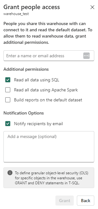

Figure 10: Sharing a Fabric warehouse

ALT: the sharing window for a warehouse in Fabric. You can change settings for additional permissions and enter e-mail addresses for adding people, just like in OneDrive.

Conclusion

Even though the storage layer is completely different than SQL Server, the Fabric warehouse is very similar to its on-premises counterpart. You can write the same T-SQL – albeit with some restrictions – and use the same security and transactions controls. The primary developer skill set is still T-SQL, combined with maybe Pipelines or Dataflows for ingesting data or for orchestrating the ETL flow. People who have been building data warehouses with relational databases should have little trouble working with the Fabric warehouse.

The Lakehouse

Together with the rise (and fall?) of big data, the data lake made its introduction years ago. Because storage is cheap, you can put terabytes of data in your data lake and figure out what to do with it later (schema-on-read vs schema-on-write). Decoupling storage from compute (in traditional databases the storage is proprietary and included into the database engine) had the advantage that you could scale your storage separately and choose which compute service suits you best. Turns out querying all those files – without any predefined structure – is quite hard. To bring together the strengths of the data lake and the traditional data warehouse, the data lakehouse was introduced. Thanks to the delta format, you can treat Parquet files like regular tables and have a transaction log associated with them. But they’re still files on a file system, so you can keep on scaling that storage.

Fabric also has a lakehouse service and as mentioned before, data is kept in the OneLake storage layer.

Tables & Files

A big difference with the warehouse is that a lakehouse can have both tables and files. Tables can be delta tables, but other types of tables are supported as well (for example csv or Parquet; a delta table is indicated with a small black triangle). Tables can be either managed (Spark takes care of the metadata and the data) or unmanaged (Spark only takes care of the metadata). A good overview of the different types is given in the article Working with tables in Microsoft Fabric Lakehouse – Everything you need to know!.

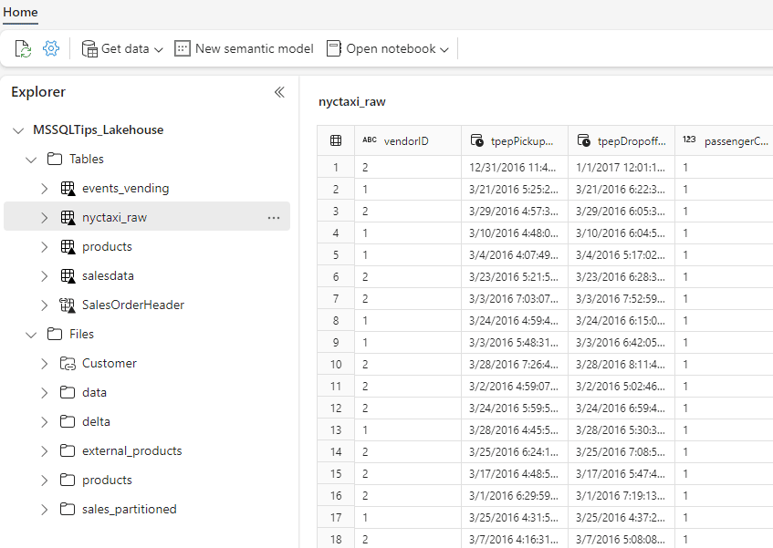
Figure 11: A lakehouse with both tables and files

ALT: a lakehouse with a table and files section. A table is selected, and its data is shown in a preview

The files section shows the “unmanaged” section of the lakehouse. This can be any file type. When you click on a folder in the explorer pane, you’ll see all of the files listed in the preview pane on the right.

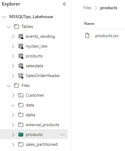
Figure 12: File preview in the lakehouse

ALT: a folder is selected in the files section of the explorer. The files in that folder are shown in the preview pane

A nice feature of Fabric is the ability to create shortcuts. With a shortcut, you can link to data that is stored in an external location, such as an Azure Blob container, an S3 bucket or maybe files in another lakehouse.

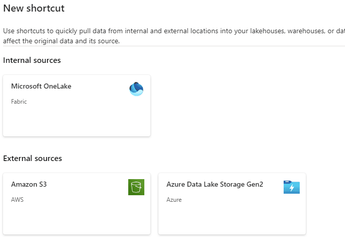
Figure 13: Dialog for creating a new shortcut

ATL: the screen you get when creating a new shortcut. You can choose between OneLake, S3, or Azure Data Lake Storage

A shortcut makes the data or file visible in the lakehouse, but it doesn’t take a physical copy. The data remains at the source and is only loaded when the shortcut is queried. Shortcuts are a method of simplifying ETL and minimizing the amount of data that needs to be copied between systems. You can create shortcuts in the file section, or you can create them in the table section. When an object is a shortcut, a little paperclip icon will be shown.

Ingesting Data

Like in the warehouse, there are a couple of ways to get data into the lakehouse.

• Pipelines and Dataflows. Exactly the same as in the warehouse, but now with a lakehouse as the destination.
• The lakehouse interface. When you right-click on a file or folder, you can choose to load its data to a (delta) table. This is fine for a one-shot analysis or a demo/proof-of-concept, but in real-life scenarios you might want to opt for an ingestion method that can be automated.

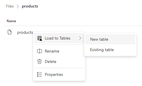
Figure 14: Load data manually to a table.

ALT: the context menu to load a file to a table in the lakehouse

• Notebooks. The main method to work with a lakehouse is notebooks. They allow you to write Spark code (PySpark, Spark SQL, Scale or SparkR). You can connect to any data source that is supported by any of the languages (you can load modules for extra functionality) and load the data to the lakehouse. In a notebook, you can control if data ends up in a delta table or another type of table, or if the table is managed or unmanaged.

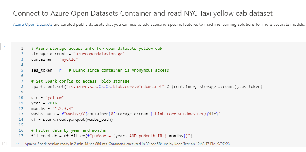
Figure 15: a notebook reading data from Azure Open Datasets with PySpark into a data frame.

ALT: a notebook with PySpark code that reads data from a blob container into a data frame

• Real-time streaming with event streams. Event streams are a low-code solution to fetch real-time data, apply rules to it and push it to one or more destinations. A lakehouse is one of the possible destinations.

Figure 16: A sample event stream in Fabric

ALT: an event stream fetching data from a sample real-time data stream, pushing the data to a lakehouse

Querying Data

Besides ingesting data, with notebooks you can also pull data into data frames, do transformations on that data and even visualize it using many of the available Python libraries. You can use Pandas data frames if you want, or use Spark SQL to write SQL queries on top of your data. Since you’re using notebooks, you can even go further and make machine learning models and do data science experiments.

Figure 17: notebook working with predictions

ALT: a notebook cell containing pyspark code

Important to note is that when you create a lakehouse, a SQL analytics endpoint is automatically created. This endpoint allows you to write T-SQL statements on top of the tables in the lakehouse, but it is read-only. This version of SQL is pretty much the same as the one you use in the warehouse, so it is a bit different from the Spark SQL you use in the notebooks. When you’re in the lakehouse, you can switch to the SQL endpoint in the top right corner:

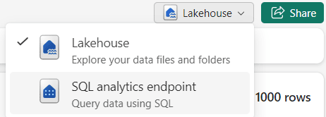
Figure 18: Switch from Lakehouse to SQL analytics endpoint

ALT: Switch from Lakehouse to SQL analytics endpoint

The SQL analytics endpoint resembles the warehouse explorer:

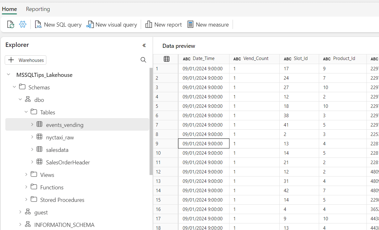
Figure 19: the SQL analytics endpoint of a lakehouse

ALT: the SQL analytics endpoint of a lakehouse. On the left there’s an object explorer, similar to the warehouse. On the right is the data preview pane.

You can write T-SQL statements just like in the warehouse (but only read-only queries):

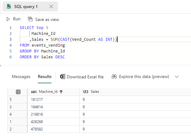
Figure 20: A T-SQL Query executed on a lakehouse

ALT: a T-SQL query executed on a lakehouse. At the bottom the result grid is shown.

The SQL endpoint is in fact treated as similar to the warehouse in the official documentation, as explained in the article Better together: the lakehouse and warehouse.

Transactions

The SQL endpoint has the same transaction support as the warehouse, but for read-only queries. This means for example that if a table has new rows added by another transaction (from a notebook), they are not included in any open transaction of running queries on the endpoint.

In theory the lakehouse supports ACID transactions because there’s a transaction log created by the delta layer. However, since it is completely open, no-one is stopping you from connecting to the OneLake storage layer and randomly deleting Parquet files from the table. This means consistency cannot be guaranteed (an interesting discussion about this topic is presented in the blog post ACID Transaction in Fabric?, and also check out the accompanying Twitter discussion).

Security

Again, the SQL analytics endpoint follows the warehouse closely. When it comes to security, the endpoint supports the same features: object and row level security is available. However, there are no such security features when working with Spark. Security is mainly defined through workspace roles and lakehouse sharing.

Conclusion

The main point I’m trying to make about the lakehouse is that it is a different beast than the warehouse. You can use notebooks to write code in various languages (PySpark, Spark SQL, Scala, SparkR and Java) and there are more possible use cases in the lakehouse, such as machine learning, data science and data visualization.

Each lakehouse comes with a SQL analytics endpoint, which you can use to write T-SQL on the lakehouse tables. The SQL endpoint shares the same features as the warehouse but is read-only.

Choosing between the Two

We’re at the end of the article and hopefully you now have a good idea which features the warehouse or the lakehouse brings. When you need to decide which service you want to use when building your data platform in Fabric, you can ask yourself any of the following questions:

• What are the skills of my current team? If you have a seasoned data warehouse team that has been building data warehouses in databases like SQL Server for years (and thus they have good SQL skills), you might want to opt for the warehouse (typical job titles are BI Developer, Analytics Engineer, ETL/data warehouse developer, data engineer). If on the other hand most people on the team have Python skills, the lakehouse might be a better option (typical job titles are data engineer and data scientist).
• Do I need to migrate existing solutions? If you have data warehouses that need to be migrated (for example from SQL Server, Azure SQL DB or Synapse Analytics), the warehouse might be the easiest option since most of the code can be migrated without too much hassle (don’t forget to check the T-SQL limitations in Fabric!). If you need to migrate solutions from Databricks, the lakehouse is the better option.
• Do you need to work with unstructured data? If you need to work with unstructured or semi-structured data, such as json files, images, video, audio and so on, the lakehouse is your choice.
• Do you need to support other use cases besides just data warehousing? For example, if you want real-time data or machine learning models, the lakehouse will be a better fit.
• What are your transaction and security requirements? If you have strict requirements about permissions, such as row-level security, and strict transaction requirements, the warehouse is probably the best options. Skills from SQL Server can easily be reused. However, the SQL analytics endpoint of the lakehouse supports the same features.

You can find a good overview of the differences between the warehouse and the lakehouse (and other services such as Power BI Datamarts and KQL databases) in the documentation.

However, the main question you might need to ask yourself is: “Do I really need to choose?”. You can perfectly combine both services in one single data platform. You can use for example the medallion architecture where the bronze and silver layer are implemented in a lakehouse (or multiple lakehouses), and the gold layer in a warehouse. This idea is entertained in the blog post Fabric: Lakehouse or Data Warehouse? by Sam Debruyn.

As we stated in the introduction: the answer is it depends.