Are Window Functions as fast as the equivalent alternative SQL methods? In this article I’ll be exploring the performance of the window functions. After you read this article I hope you’ll be in a better position to decide whether it is really worth changing your application code to start using window functions.
Before I start the tests, I would like to explain the most important factor that affects the performance of window functions. A window spool operator has two alternative ways of storing the frame data, with the in–memory worktable or with a disk–based worktable. You’ll have a huge difference on performance according to the way that the query processor is executing the operator.
The in-memory worktable is used when you define the frame as ROWS and it is lower than 10000 rows. If the frame is greater than 10000 rows, then the window spool operator will work with the on-disk worktable.
The on-disk based worktable is used with the default frame, that is, “range…“ and a frame with more than 10000 rows.
It’s possible to check whether the window spool operator is using the on-disk worktable by looking at the results of the SET STATISTICS IO. Let’s see a small example of the window spool using the on-disk based worktable:
|
1 2 3 4 5 6 7 8 9 10 11 12 13 |
USE tempdb GO IF OBJECT_ID('tempdb.dbo.#TMP') IS NOT NULL DROP TABLE #TMP GO CREATE TABLE #TMP (ID INT, Col1 CHAR(1), Col2 INT) GO INSERT INTO #TMP VALUES(1,'A', 5), (2, 'A', 5), (3, 'B', 5), (4, 'C', 5), (5, 'D', 5) GO SET STATISTICS IO ON SELECT *, SUM(Col2) OVER(ORDER BY Col1 RANGE UNBOUNDED PRECEDING) "Range" FROM #TMP SET STATISTICS IO OFF |
|
1 2 |
Table 'Worktable'. Scan count 5, logical reads 29, physical reads 0, read-ahead reads 0, lob logical reads 0, lob physical reads 0, lob read-ahead reads 0. Table 'Worktable'. Scan count 1, logical reads 1, physical reads 0, read-ahead reads 0, lob logical reads 0, lob physical reads 0, lob read-ahead reads 0. |
|
1 2 3 4 |
SET STATISTICS IO ON SELECT *, SUM(Col2) OVER(ORDER BY Col1 ROWS UNBOUNDED PRECEDING) "Rows" FROM #TMP SET STATISTICS IO OFF |
|
1 2 |
Table 'Worktable'. Scan count 0, logical reads 0, physical reads 0, read-ahead reads 0, lob logical reads 0, lob physical reads 0, lob read-ahead reads 0. Table 'Worktable'. Scan count 1, logical reads 1, physical reads 0, read-ahead reads 0, lob logical reads 0, lob physical reads 0, lob read-ahead reads 0. |
As you can see, the worktable has some reads when you use a “range”, but it doesn’t happen with the in-memory worktable which is used when you use “Rows”.
Optionally you also can look at the xEvent called window_spool_ondisk_warning. Fortunately on SQL Server 2012 we’ve a very nice interface that we can use to deal with xEvents. In SSMS, you can easily capture an event, and then look at the live data captured. Here you can see a screen-capture of this interface:
 |
 |
There are many aspects of the window spool operator that could be improved, I just opened some connect items about this and I’d appreciate it if you could take a minute or so to vote on this items.
- Window Spool worktable doesn’t spill to tempdb
- Default window spool worktable in memory
- Granting memory to process window spool worktable
- Unnecessary Sort
For now, when the logic of the query allows it, it is a good practice to always define the window frame as ROWS in order to try to use the in-memory worktable.
Performance tests
I’ll now show some performance tests that I did with the most-used windows functions such as LEAD, LAG, LAST_VALUE and the OVER clause.
To execute the tests, I used the free SQLQueryStress toll created by Adam Machanic (blog | twitter), you can download it here, I also will use the sample database AdventureWorks2008R2.
Let’s start by testing the performance of the clause OVER with the running aggregation solution, let’s see how it would scale with many users demanding information from the server.
First let’s create a table with 453772 rows:
|
1 2 3 4 5 6 7 8 9 10 11 12 13 14 15 16 17 18 19 20 21 |
USE AdventureWorks2008R2 GO SET NOCOUNT ON; IF OBJECT_ID('TestTransactionHistory') IS NOT NULL DROP TABLE TestTransactionHistory GO SELECT IDENTITY(INT, 1,1) AS TransactionID, ProductID, ReferenceOrderID, ReferenceOrderLineID, TransactionDate, TransactionType, Quantity, ActualCost, ModifiedDate INTO TestTransactionHistory FROM Production.TransactionHistory CROSS JOIN (VALUES (1), (2), (3) , (4)) AS Tab(Col1) GO CREATE UNIQUE CLUSTERED INDEX ixClusterUnique ON TestTransactionHistory(TransactionID) GO |
Running Aggregation, Clause OVER + Order By
Now let’s run the old solution to the running aggregation query:
|
1 2 3 4 5 6 7 8 9 10 11 12 13 14 15 16 |
-- Creating a index to help the subquery CREATE INDEX ix1 ON TestTransactionHistory (ProductID, TransactionDate) INCLUDE(Quantity) -- Old Solution -- Test running 200 threads, 5 iterations per session -- AVG Elapsed time: 00:02:02.3009 -- AVG Logical Reads: 8665 SELECT TransactionID, ProductID, Quantity, (SELECT SUM(Quantity) FROM TestTransactionHistory b WHERE b.ProductID = a.ProductID AND b.TransactionDate <= a.TransactionDate) AS "Running Total" FROM TestTransactionHistory a WHERE ProductID = ROUND(((999 - 930 -1) * RAND() + 930), 0) GO |
Let’s look at the execution plan:
This is a pretty straightforward plan: For each row read in the table, it executes the seek to calculate the running totals.
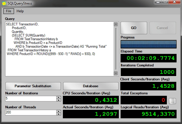
I’m filtering by a random ProductID to simulate many users requiring different products at the same time. Let’s run it in on SQLQueryStress:
Now let’s run it using the clause OVER with ORDER BY:
|
1 2 3 4 5 6 7 8 9 10 |
-- Clause Over with ORDER BY, DEFAULT FRAME RANGE UNBOUNDED PRECEDING -- Test running 200 threads, 5 iterations per session -- AVG Elapsed time: 00:00:14.5668 -- AVG Logical Reads: 8957 SELECT TransactionID, ProductID, Quantity, SUM(Quantity) OVER (PARTITION BY ProductID ORDER BY TransactionDate, TransactionID RANGE UNBOUNDED PRECEDING) "Running Total" FROM TestTransactionHistory WHERE ProductID = ROUND(((999 - 930 -1) * RAND() + 930), 0) GO |
The execution plan is:
As you can see, there is no double access to the table here. There is just a window spool doing the magic of keeping the rows to be aggregated.
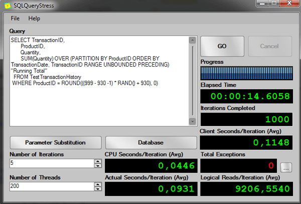
The results from SQLQueryStress:
Now let’s specify the ROWS frame in the query and run again:
|
1 2 3 4 5 6 7 8 9 10 |
-- Clause Over with ORDER BY, ROWS WINDOW FRAME, ROWS UNBOUNDED PRECEDING -- Test running 200 threads, 5 iterations per session -- AVG Elapsed time: 00:00:02.7381 -- AVG Logical Reads: 8 SELECT TransactionID, ProductID, Quantity, SUM(Quantity) OVER (PARTITION BY ProductID ORDER BY TransactionDate, TransactionID ROWS UNBOUNDED PRECEDING) "Running Total" FROM TestTransactionHistory WHERE ProductID = ROUND(((999 - 930 -1) * RAND() + 930), 0) GO |
The results from SQLQueryStress:
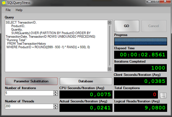
As you can see in the elapsed time, the difference between the old solution and the solution using the worktable is very good.
|
Query |
Client Seconds/Iteration (Avg) |
CPU Seconds/Iteration (Avg) |
Actual Seconds/Iteration (Avg) |
Logical Reads/Iteration (Avg) |
|
old solution |
0,4312 |
1,4528 |
1,2097 |
9514,3370 |
|
RANGE query |
0,1148 |
0,04 |
0,0931 |
9206,5540 |
|
ROWS query |
0,0385 |
0,0075 |
0,0241 |
9,0800 |
What about the LEAD and LAG function?
LEAD
First let’s see the execution plan for a query to return the next row from the TransactionHistory table.
|
1 2 3 4 5 6 7 8 9 10 11 12 13 14 15 16 |
-- Old Solution -- Test running 50 threads, 5 iterations per session -- AVG Elapsed time: 00:00:33.7419 -- AVG Logical Reads: 11860 SELECT a.TransactionID, Tab."Next TransactionID" a.ProductID FROM TestTransactionHistory a OUTER APPLY (SELECT TOP 1 b.TransactionID AS "Next TransactionID" FROM TestTransactionHistory b WHERE b.ProductID = a.ProductID AND b.TransactionID > a.TransactionID ORDER BY b.TransactionID) AS Tab WHERE a.ProductID = ROUND(((999 - 930 -1) * RAND() + 930), 0) ORDER BY a.ProductID, a.TransactionID GO |
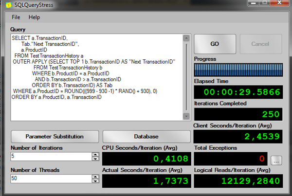
As you can see, an easy way to do get the next row of a table is using the OUTER APPLY clause. Let’s see the performance of this query:
Now let’s see the same query but now using the LEAD function to get the next row.
|
1 2 3 4 5 6 7 8 9 10 |
-- Using LEAD function -- Test running 50 threads, 5 iterations per session -- AVG Elapsed time: 00:00:00.9020 -- AVG Logical Reads: 9 SELECT TransactionID, LEAD(TransactionID) OVER(ORDER BY ProductID, TransactionID) AS "Next TransactionID", ProductID FROM TestTransactionHistory WHERE ProductID = ROUND(((999 - 930 -1) * RAND() + 930), 0) ORDER BY ProductID, TransactionID |
Execution Plan:
As you can see from the execution plan, we could improve the query by creating an index on the columns ProductID and TransactionID to remove the sort operator, but in order to compare the performance, let’s see the results of the execution on this query:
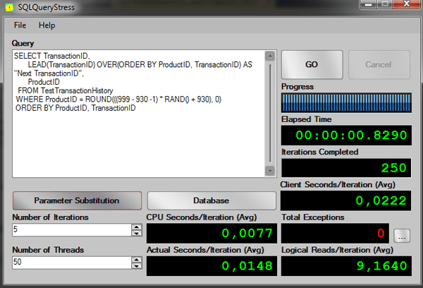
Again, the window function is much better than the old subquery solution.
|
Query |
Client Seconds/Iteration (Avg) |
CPU Seconds/Iteration (Avg) |
Actual Seconds/Iteration (Avg) |
Logical Reads/Iteration (Avg) |
|
Subquery solution |
2,4539 |
0,4108 |
1,7373 |
12129,2840 |
|
Window Function |
0,0222 |
0,0077 |
0,0148 |
9,1640 |
Now let’s see the LAG function.
LAG
First the old approach to get the previews row:
|
1 2 3 4 5 6 7 8 9 10 11 12 13 14 15 16 |
-- Old Solution -- Test running 50 threads, 5 iterations per session -- AVG Elapsed time: 00:00:31.4037 -- AVG Logical Reads: 11125 SELECT a.TransactionID, Tab."Previews TransactionID" a.ProductID FROM TestTransactionHistory a OUTER APPLY (SELECT TOP 1 b.TransactionID AS "Previews TransactionID" FROM TestTransactionHistory b WHERE b.ProductID = a.ProductID AND b.TransactionID < a.TransactionID ORDER BY b.TransactionID DESC) AS Tab WHERE a.ProductID = ROUND(((999 - 930 -1) * RAND() + 930), 0) ORDER BY a.ProductID, a.TransactionID GO |
The results from SQLQueryStress:
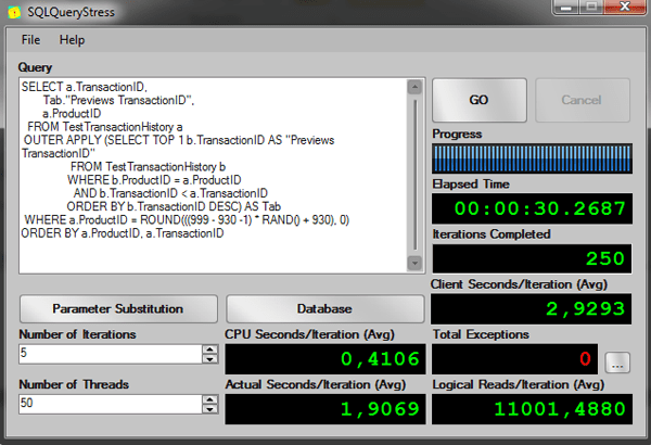
Now using the LAG function:
|
1 2 3 4 5 6 7 8 9 10 |
-- Using LAG function -- Test running 50 threads, 5 iterations per session -- AVG Elapsed time: 00:00:00.8690 -- AVG Logical Reads: 9 SELECT TransactionID, LAG(TransactionID) OVER(ORDER BY ProductID, TransactionID) AS "Previews TransactionID" ProductID FROM TestTransactionHistory WHERE ProductID = ROUND(((999 - 930 -1) * RAND() + 930), 0) ORDER BY ProductID, TransactionID |
The results from SQLQueryStress:

Once again, the performance on windowing functions is much better.
|
Query |
Client Seconds/Iteration (Avg) |
CPU Seconds/Iteration (Avg) |
Actual Seconds/Iteration (Avg) |
Logical Reads/Iteration (Avg) |
|
Subquery solution |
2,9293 |
0,4106 |
1,9069 |
11001,4880 |
|
Lag Window function |
0.0193 |
0,0062 |
0,0117 |
8,2160 |
Note: The LEAD and LAG functions doesn’t accept a frame, in this case the default of window spool is to use the in memory worktable.
First_Value and Last_Value
Let’s suppose I want to return all the employees from a specific department. I also want to know which employee had the largest number of hours not working because he/she was sick and who that employee was.
To write it without window functions, I could use subqueries to return the data of most hours sick and who was the employee; something like the following query:
|
1 2 3 4 5 6 7 8 9 10 11 12 13 14 15 16 17 18 19 20 21 22 23 24 25 26 27 28 29 30 31 32 33 34 35 |
-- Old Solution -- Test running 200 threads, 100 iterations per session -- AVG Elapsed time: 00:00:14.7488 -- AVG Logical Reads: 391 DECLARE @i INT = ROUND(((16 - 1 -1) * RAND() + 1), 0); WITH CTE_1 AS ( SELECT Person.FirstName + ' ' + Person.LastName AS EmployeeName, Employee.JobTitle, Employee.SickLeaveHours, Employee.HireDate, Department.Name AS DepartmentName FROM HumanResources.Employee INNER JOIN HumanResources.EmployeeDepartmentHistory ON Employee.BusinessEntityID = EmployeeDepartmentHistory.BusinessEntityID INNER JOIN HumanResources.Department ON EmployeeDepartmentHistory.DepartmentID = Department.DepartmentID INNER JOIN Person.Person ON Employee.BusinessEntityID = Person.BusinessEntityID WHERE EmployeeDepartmentHistory.EndDate IS NULL AND Department.DepartmentID = @i ) SELECT a.*, (SELECT TOP 1 b.SickLeaveHours FROM CTE_1 b WHERE a.DepartmentName = b.DepartmentName ORDER BY b.SickLeaveHours DESC) AS MostSickEmployee, (SELECT TOP 1 c.EmployeeName FROM CTE_1 c WHERE a.DepartmentName = c.DepartmentName ORDER BY c.SickLeaveHours DESC, c.HireDate DESC) AS MostSickEmployeeName FROM CTE_1 a ORDER BY a.DepartmentName, a.EmployeeName GO |
This is the result:
The employee that had the most time off-sick was “Brian LaMee”. I had to use a CTE to make the query a little easier to understand, and I wrote two subqueries on this CTE.
Let’s see the performance:
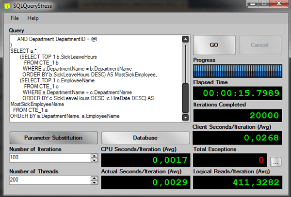
Now how it would be with window functions?
When you first try the functions FIRST_VALUE and LAST_VALUE, it may seem confusing and you might wonder if the functions MAX and MIN wouldn’t return the same values of FIRST_VALUE and LAST_VALUE, let’s see an example.
|
1 2 3 4 5 6 7 8 9 10 11 12 13 14 15 16 17 18 19 20 21 |
-- New Solution -- Test running 200 threads, 100 iterations per session -- AVG Elapsed time: 00:00:11.9196 -- AVG Logical Reads: 189 SELECT Person.FirstName + ' ' + Person.LastName AS EmployeeName, Employee.JobTitle, Employee.SickLeaveHours, Employee.HireDate, Department.Name AS DepartmentName, MAX(Employee.SickLeaveHours) OVER(PARTITION BY Department.Name ORDER BY Employee.SickLeaveHours ROWS BETWEEN UNBOUNDED PRECEDING AND UNBOUNDED FOLLOWING) AS MostSickEmployee, LAST_VALUE(Person.FirstName + ' ' + Person.LastName) OVER(PARTITION BY Department.Name ORDER BY Employee.SickLeaveHours, Employee.HireDate ROWS BETWEEN UNBOUNDED PRECEDING AND UNBOUNDED FOLLOWING) AS MostSickEmployeeName FROM HumanResources.Employee INNER JOIN HumanResources.EmployeeDepartmentHistory ON Employee.BusinessEntityID = EmployeeDepartmentHistory.BusinessEntityID INNER JOIN HumanResources.Department ON EmployeeDepartmentHistory.DepartmentID = Department.DepartmentID INNER JOIN Person.Person ON Employee.BusinessEntityID = Person.BusinessEntityID WHERE EmployeeDepartmentHistory.EndDate IS NULL AND Department.DepartmentID = ROUND(((16 - 1 -1) * RAND() + 1), 0) ORDER BY Department.Name, Person.FirstName + ' ' + Person.LastName |
And the results:
The same results were returned, and the in fact the function MAX can be used to return the LAST_VALUE of the value in a partition, in this case the partition is the department, so the MAX of a window partitioned by department with a frame that goes from UNBOUNDED PRECEDING AND UNBOUNDED FOLLOWING will return the last value based on the ORDER BY of the column specified in the MAX function.
The LAST_VALUE function will return the last value based on the ORDER BY clause specified in the OVER clause. If you didn’t understand, then try to change the LAST_VALUE for the MAX and see that the results will not be the ones you might expect.
Now let’s see the performance:
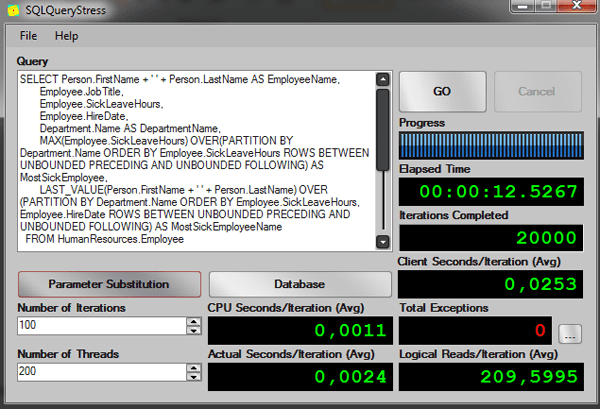
This time we can’t see a big difference between the queries, but that’s probably because the tables I used are very small.
|
Query |
Client Seconds/Iteration (Avg) |
CPU Seconds/Iteration (Avg) |
Actual Seconds/Iteration (Avg) |
Logical Reads/Iteration (Avg) |
|
CTE solution |
0,0268 |
0,0017 |
0,0029 |
411,3282 |
|
Window function |
0,0253 |
0,0011 |
0,0024 |
209,5995 |
Note: The performance will vary in your SQL Server environment since the codes are all random.
Conclusion
In general the window functions will perform better than the old solutions using subqueries that we are used to writing.
I recommend you to always test both solutions the old and the new using the window function, if the new solution is not performing better than the old one you should always check whether the window spool operator is working with the worktable on-disk.
That’s all folks.


Load comments