In Parts I (Solving the Overlap Query Problem in PostgreSQL) and II (Overlapping Ranges in Subsets in PostgreSQL) of this series, we used the GiST index type – and its lesser known cousin: SP-GiST – to turbocharge the performance of overlap queries. But GiST indexes are extremely versatile, with uses far beyond the examples I have used so far.

In this final article, we’ll explore some of the many other ways they can be used.

Stuck in the Middle With You

We’ve used only one operator in all our queries so far: the “&&” operator, which returns true if two ranges overlap to any degree. There are other range operators that GiST can use to accelerate query performance. The operators “<<” and “>>” determine whether one range is entirely to the left or the right of another. These aren’t terribly interesting, as an ordinary B-Tree index can easily support the same type of query.

More useful are the inclusion operators  ‘<@‘  and ‘ @>‘. These tell you if the first range lies entirely inside the second or vice versa. To illustrate their use, consider our Part I example of museum patrons and security outages. (If you haven’t been following, along, the code to create these objects is in the Appendix of Part II)

Our original query identified patrons who were present during some portion of an outage (any amount of overlap). But to find patrons who were present for an entire outage (the outage both began and ended during their visit) we write this query:

Conversely, to locate patrons who arrived and left during an outage (their visit lies entirely inside the outage), either reverse the order of operands in the WHERE clause or change the operator to point the other direction:

It’s easy to remember these operators using the same rule taught in elementary school math: the little end of the “<” and “>” signs points to the smaller range.

These operators will work without any index being defined, but the query will be extremely slow. If we rewrite the query using standard ‘<' and ‘>‘ operators, an ordinary B-Tree index will provide some help:

But the performance gains from a GiST index can be astronomical. Running the above queries on our Part I/II test data yields the following results.

Reminder: our test data is well-suited to SP-GiST. Against data sets with more overlap, GiST may perform better.

The Query from Another Dimension

So far we’ve only used GiST with one-dimensional data: date and timestamp ranges. GiST becomes even more useful with two-dimensional queries. If you think to yourself, “I don’t have exotic queries like that: just ordinary dates and numbers”, well you’re likely to be surprised.

To explain, let’s create a new set of test data: a table tracking sales of some (unnamed) commodity. Our table has four columns: a customer_id, the sale date, and the bid price and ask price.

Note: if you want to test this code on your own computer, there is code to generate a set of data in the appendix of this article, in the section of code named: — Script to test bid/ask queries. The data is randomized, so your output will not match exactly, but should be very close in usage.

Let’s assume we want to find sales where the bid price lies in a certain range and the sale price lies in another:

This is a two-dimensional query; the value range for bid price is one dimension, while ask price is the other. To better visualize this, let’s first examine a basic 2-D geographic query, the type GiST is commonly used for: finding a set of points that lie within a ‘box” of latitude/longitude values.

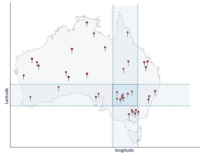
B-Tree indexes perform badly here. They can quickly locate one range – either the latitude or the longitude band show above – but then they’re forced to scan for the intersection with the other band.

Now let’s translate this concept to our commodity sales query. Just like our geographic query, we have two “bands” of values our query needs to intersect, bid price and ask price:

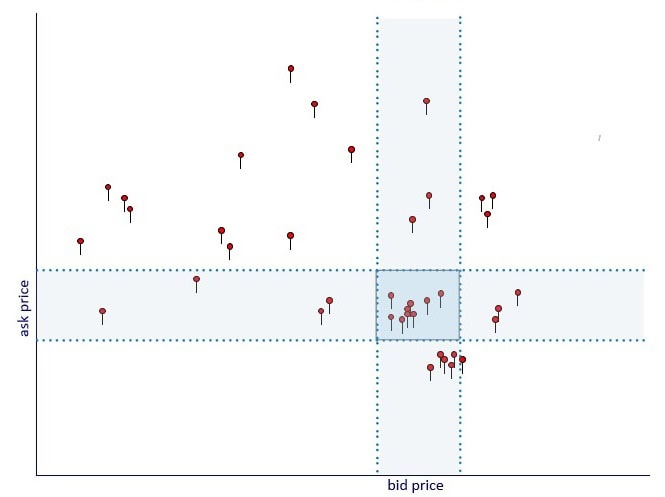
The intersection “box” isn’t a geographic region on a map, but it still lies within a two-dimensional space. And GiST absolutely loves queries like this. B-Trees use a one-dimensional structure, but GiST uses a two-dimensional analogue known as an R-Tree (SP-Gist uses a similar quadtree).

Let’s rewrite our bid/ask price query to use GiST. Since we’re searching for two-dimensional points, we create an index using a POINT object, with bid price as one coordinate, and ask price the other:

To perform the actual search, we match this point to our desired search “box”. PostgreSQL’s default box() function only accepts points though. To simplify the syntax, we define a box() function that accepts four numeric values:

Now we can write our search query. The “<@” inclusion operator finds points within a box. This query finds all rows with bid price between $600 and $620 and ask price between $615 and $625:

OK, it works – but are the results worth dealing with this opaque syntax? How much faster is it than the traditional BETWEEN syntax and an ordinary B-Tree index? Let’s run some timings! (The queries and indexes used for these tests are included in the Appendix)

The table below shows benchmark results for the various index types. Three different query parameter scenarios are tested, all returning the same number of rows. In the balanced scenario, the range of values for both search terms (bid and ask price) are equal. This corresponds to the horizontal and vertical search bands in the above image being equal width – each range by itself matches 0.3% of the table’s 50M rows.

The “favored” scenario divides the range of bid values by a factor of six, while multiplying the ask range by the same amount. This selects the same amount of data, but now the bid price is doing nearly all the work of filtering. If the table contains a B-Tree index starting with bid price, this is the best-case scenario. Similarly, the “adverse” query reverses this, widening bid price range by 6X and narrowing ask price similarly.

There’s a lot of information to unpack here. With no index, all three queries have identical (terrible) performance. An index on just one search term (bid price) doesn’t help much: the “favored” scenario sees a slight speed boost, but the adverse query fails to use the index entirely, while the balanced scenario actually slows down. Ouch.

A compound index on both bid and ask does much better performance-wise, but it is very sensitive to the search terms, with performance varying by more than a factor of 3 from the slowest to the fastest query. In the adverse scenario, the bid price range matches 900K of our 50M rows – compound B-Tree indexes perform poorly when their primary term isn’t very selective.

Our GiST index shines here. It ties the B-Tree in the favored scenario, is 50% faster on balanced queries, and a full 3.4X faster on the “adverse” scenario. More importantly, the performance of the GiST index is much more consistent. Between the favored to the adverse scenario the specificity of the search values changes by a factor of 36, yet the query time barely changes. This is the predictable behavior we want from an index.

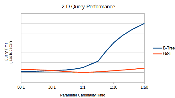
SP-GiST is also consistent on performance, but offers no advantage over basic GiST, and in fact is slightly slower in two of three scenarios. But hold tight: SP-GiST has an advantage that we’ll see below.

We could improve worst-case B-Tree performance by creating a second index, reversing the column order to “ask, bid”. But maintaining two indexes requires double the cost and storage and performance still wouldn’t match our single GiST index. And as the table increases in size, the B-Tree index will fall further behind.

Like an ordinary index, a two-dimensional GiST index can be made compound by adding additional columns. For instance, if we our bid/ask query needs to search for a specific commodity code, we can include this column in our index (note that this column does not exist in this table and is just an example. This type of index requires the btree-gist extension mentioned in Part II):

What if our query has more than two range parameters? Three ranges would turn our search box into a 3-D cube; four ranges a 4-D hypercube, etc, etc. Extending our 2-D approach to higher dimension indexes is possible, but beyond the scope of this article.

Luckily this is rarely necessary. A 2-D index on the two ‘best’ parameters (those with the highest cardinality) usually winnows the result set enough that a simple scan on the remaining criteria is fast enough.

A Warm Fuzzy Search

If the above results don’t convince you there’s value in a 2-D GiST query, let’s look at another type of query they accelerate … and by an even larger margin. This is the so-called kNN “nearest neighbor” search. Queries like this allow us to ‘fuzzily’ match multiple search criteria, returning the closest values found.

Using our sales table example, let’s assume we want the best match to a bid price of $570 and an ask price of $575. Either price can vary from our desired value; what we want are rows that have the least difference in both values simultaneously.

Writing this in standard SQL is messy, but PostgreSQL has a built-in operator to find the distance between points, the “<->” operator. Using the point() syntax from above, we can find closest matches by ordering off the results of this operator. Then we simply limit the query results to the number of “fuzzy” matches desired. For instance, the “LIMIT 1” in this query finds the single best match:

For the best “n” matches, increase the LIMIT accordingly. Ordering the table in reverse (descending order) would give you the worst matches, though uses for this are rare (searches on an “opposites attract” dating site, perhaps?)

Queries like this don’t specifically require a GiST index, but performance will be abysmal for all but very small data sets:

Here, SP-GiST outshines its bigger brother, turning in nearly 30% better performance than GiST, and well over 1000x faster than the un-utilized B-Tree index. That’s speed worth working for.

The “<->” operator calculates “Euclidean” distance – using the Pythagorean theorem from junior high school – meaning that if both prices differ by $10, the distance becomes 14.1, not 20. It also weights both search criteria equally. If we wanted our fuzzy search to be more sensitive to differences in bid price than ask price, we could scale the value accordingly when creating the point object (though we need to perform the same scaling when creating the index.)

A Date With Destiny

Multidimensional queries aren’t limited to numeric values. With a little effort, we can include dates, even querying a date range in conjunction with a numeric one. Using our sample sales table, let’s try to write the following query to be usable by a 2-D GiST index:

Again there are two independent ranges of values – one a date, the other numeric – that jointly comprise a 2-dimensional query. To use a GiST index with this, we need to be able to create point() and box() objects, but these functions require numeric arguments. The easiest way to do this is to subtract from each date an (arbitrary) fixed date, transforming the original value into the number of days elapsed. We could do this directly, but it will simplify the syntax if we create another helper function. The unimaginatively named “day_cnt()” returns the number of days since Jan 1, 2000:

Now index on a point() object containing the sales date and bid price:

To use the index, pass the query dates to our helper function as part of constructing the query box:

This syntax is still convoluted, but if you use it often, you can define point() and box() helper functions that accept dates directly, making it just about as straightforward as a standard SQL query.

Performance for this query is similar to the bid/ask scenarios we ran above: tying a B-Tree index when the first parameter range is tiny compared to the second, and several times faster in the reverse case. And we can also perform fuzzy matches on dates. This query finds the three closest matches to a sale made Aug 10,2024 for $500:

Reminder: the closest matches are based on date and price; both can vary at once. Because we’re converting sale date to a count of days, every $1 difference in bid price equates to 1 day difference in sale date, i.e. the two rows below are equally “far” from our search criteria:

sdate: 08-15-2024 bid price: $500 (14 day difference)

sdate: 08-01-2024 bid price: $514 ($14 difference)

If we modify day_cnt() to return the number of weeks, then a $1 price difference equates to a sale date difference of one week. Alternately, if we divide bid price by 10 before indexing, everyday difference in sale date equates to a $10 price difference.

Conclusion

Even after three articles on the subject, we’ve just scratched the surface of what’s possible with flexible, multi-purpose GiST indexes. The next time you’re faced with a tough index strategy challenge, stop to consider if GiST may provide a solution.

Appendix I — test data script